Time Series Clustering: Unleashing Patterns in Financial Markets
Introduction to Time Series Clustering
Welcome to a journey through time and data. This adventure takes us through the intricate paths of Time Series Clustering, a crucial tool that financial analysts and investors use to uncover hidden patterns in temporal data. Hold tight as we delve into this exciting area of Data Science and Artificial Intelligence, particularly in Indian Financial Equity Markets.
Time Series Clustering
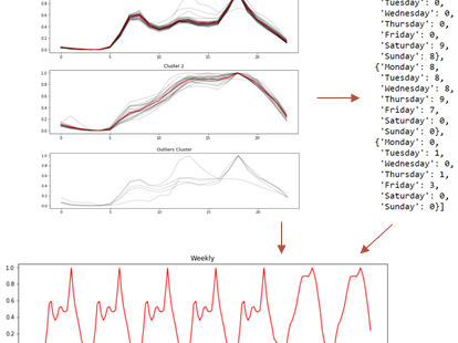
In the realm of financial markets, time series clustering stands as a potent tool. It takes sequences of data points, recorded over time, and groups them based on similarity. Two key methods employed in this process include Hierarchical Clustering and DBSCAN Clustering.
Hierarchical Clustering, a type of agglomerative clustering, starts by treating each data point as a separate cluster. It then progressively merges the clusters based on their distance, creating a tree of clusters known as a dendrogram. This method allows us to visualize the clusters and their relationships, providing valuable insights into our data structure.
DBSCAN, short for Density-Based Spatial Clustering of Applications with Noise, operates on a different principle. This density-based clustering algorithm defines clusters as high-density regions separated by areas of low density. Unlike hierarchical clustering, DBSCAN does not require us to specify the number of clusters beforehand, making it useful for discovering clusters of arbitrary shape in our data.
Application in Finance
Time series clustering finds a significant place in the financial market. Its main strength lies in its ability to unravel patterns and trends in stock prices. This becomes particularly crucial in Indian Equity Markets, known for their vibrant and dynamic nature.
Consider the daily closing prices of various stocks. Time series clustering allows us to group these stocks based on the similarity of their price movements. We may find that stocks in the same sector, such as IT or healthcare, fall into the same cluster due to similar market influences.
Limitations
Despite its immense utility, time series clustering comes with challenges. A key limitation lies in the dependence on the quality of data and the choice of distance measure and clustering algorithm. Noise in the data or an ill-suited distance measure can lead to misclassification of data points, resulting in less meaningful clusters.
Additionally, the outcome of clustering can vary with different parameters. The same data set can yield different clusters with a different number of clusters in hierarchical clustering or a different density threshold in DBSCAN. Therefore, carefully selecting and fine-tuning parameters become essential for reliable clustering results.
Case Study
Let's consider a case study to bring the concepts discussed to life. We take a dataset of daily closing prices for various stocks listed on the BSE and NSE over the past year. We then apply time series clustering to group these stocks.
1️⃣ First, we collect and preprocess the data, handling missing values and normalizing the prices.
2️⃣ Next, we apply hierarchical clustering and DBSCAN to the data.
3️⃣ Finally, we visualize the clusters and analyze the results.
Upon analysis, we notice stocks from the same sector cluster together, highlighting the similarity in their price movements. For example, IT stocks like Infosys and TCS fall into the same cluster, reflecting their shared market influences.
Sample Python Code for Time Series Clustering
import pandas as p
import numpy as np
from sklearn.preprocessing import MinMaxScaler
from sklearn.cluster import AgglomerativeClustering, DBSCAN
import matplotlib.pyplot as plt

# Collect and preprocess the data
data = pd.read_csv("your_data.csv")
data.fillna(method='ffill', inplace=True)

# Normalize the prices
scaler = MinMaxScaler()
data_scaled = scaler.fit_transform(data.drop(columns=["Stock_Symbol"]))

# Apply Hierarchical Clustering
cluster = AgglomerativeClustering(n_clusters=5, affinity='euclidean', linkage='ward')
data['hierarchical_cluster'] = cluster.fit_predict(data_scaled)

# Apply DBSCA
dbscan = DBSCAN(eps=0.5)
data['dbscan_cluster'] = dbscan.fit_predict(data_scaled)

# Visualize the clusters and analyze the results
for cluster_type in ['hierarchical_cluster', 'dbscan_cluster']:
    plt.figure(figsize=(10, 7))
    plt.scatter(data["Stock_Symbol"], [0]*len(data), c=data[cluster_type])
    plt.title(f'Clusters from {cluster_type}')
    plt.show()
This script reads stock prices from a CSV file, handles missing values, and normalizes the prices. Then, it applies Hierarchical Clustering and DBSCAN to the data. Finally, it visualizes the clusters for each method.
This is a simplified example, and the parameters for the clustering algorithms (like the number of clusters for AgglomerativeClustering or the eps parameter for DBSCAN) as well as the preprocessing steps might need to be adjusted based on the specifics of your dataset and the exact requirements of your analysis.
Closing Thoughts on Time Series Clustering
Thus, through time series clustering, we unravel the patterns hidden in the financial market's ebbs and flows. We witness the power of hierarchical and DBSCAN clustering in grouping similar time series data, aiding in identifying market trends and informing investment decisions.
Yet, we must remember that time series clustering is a supplement, not a substitute, for sound financial judgment. Variability with parameters and dependence on data quality reminds us that even the most advanced tools require careful handling and human insight.
In this journey through time and data, we uncover patterns, reveal trends, and build a foundation for informed strategic decisions. Let us harness the power of time series clustering, using it to navigate the vibrant, dynamic landscape of the Financial Market.
Follow Quantace Research
-------------
Why Should I Do Alpha Investing with Quantace Tiny Titans?
1) Since Apr 2021, Our premier basket product has delivered +50.4% Absolute Returns vs the Smallcap Benchmark Index return of +11.2%. So, we added a 39% Alpha.
2) Our Sharpe Ratio is at 1.4.
3) Our Annualised Risk is 20.1% vs Benchmark's 20.4%. So, a Better ROI at less risk.
4) It has generated Alpha in the challenging market phase.
5) It has a good consistency and costs 6000 INR for 6 Months.
-------------
Disclaimer: Investments in securities market are subject to market risks. Read all the related documents carefully before investing. Registration granted by SEBI and certification from NISM in no way guarantee performance of the intermediary or provide any assurance of returns to investors.
-------------
#future #machinelearning #research #investments #markets #investing #like #investment #assurance #management #finance #trading #riskmanagement #success #development #strategy #illustration #assurance #strategy #mathematics #algorithms #machinelearning #ai #algotrading #data #financialmarkets #quantitativeanalysis #money


